Branch-Line Coupler
Introduction
This is a microstrip Branch-Line coupler designed over a 20 mil RO4003C.
The project files are available here
The Branch-Line coupler is one of the easiest couplers to design, and it is very common and well known in the literature. It consists of four λ/4 transmission lines: the series lines are Z₀/√2 Ω and the shunt lines are Z₀ Ω.
The main disadvantage of this structure is its narrow bandwidth. It can be improved by adding an extra box, but this comes with slightly higher insertion loss and, obviously more PCB area.
Features
Simple design
Easy to fabricate in microstrip
Good port isolation
Equal power split (3 dB)
90° phase difference between output ports
All ports are matched simultaneously
Warning
Narrow bandwidth (~10–20%)
Large size at low frequencies
References
David M. Pozar, Microwave Engineering, 4th Edition, 2012. Chapter 7.5
Unknown Editor, Microwaves101, Branchline Couplers
Specifications
Feature |
Value |
|---|---|
Band |
[1800, 2200] MHz |
Insertion Loss (I/Q) |
3.5 ± 0.5 dB |
I/Q phase difference |
90±2 deg |
Return Loss |
<-12 dB |
I/Q Isolation |
>12 dB |
Design Procedure
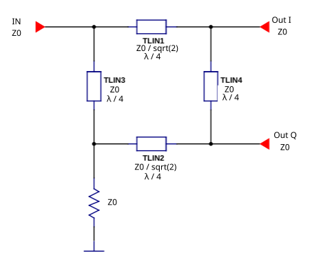
1. Ideal Transmission Line Implementation
As a first approach, the Branch-Line is designed with ideal transmission lines to see its behavior. This can be done in Qucs-S using the Qucsator-RF backend.
Branch-Line schematic with ideal transmission lines
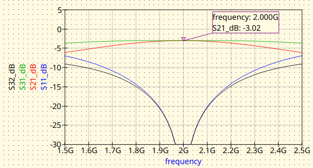
Branch-Line with ideal transmission lines. Magnitude response
Branch-Line with ideal transmission lines. Phase difference between outputs
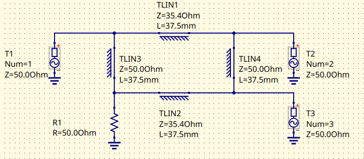
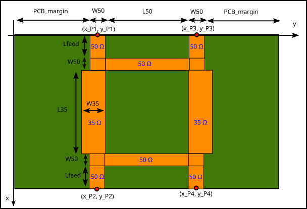
2. Microstrip (MS) Line Implementation
The ideal transmission lines are replaced by microstrip transmission lines. The synthesis can be done with the Transmission Line tool from Qucs-S or directly with the RF Circuit Synthesis Tools embedded in the Qucs-S S-Parameter Viewer, both tools are included in the Qucs-S suite.
2.1 MS: No Junctions nor Feed Lines
The ideal transmission lines by microstrip lines. The junctions and the feed lines are not included at this stage. This approach will let to evaluate the impact of the junctions and also, the feedlines later.
Branch-Line with microstrip lines. Schematic
Branch-Line with microstrip lines. Magnitude response
Branch-Line with microstrip lines. Phase difference between outputs
2.2 MS: Add Junctions and Feed Lines
The tee junctions and the feed lines are added. Notice that the tee junctions pull the center frequency down. The feed lines have no effect on the response as they are 50 Ω lines, they only add some insertion loss.
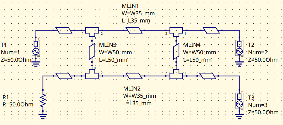
Branch-Line with microstrip lines. Schematic
Branch-Line with microstrip lines. Magnitude response
Branch-Line with microstrip lines. Phase difference between outputs
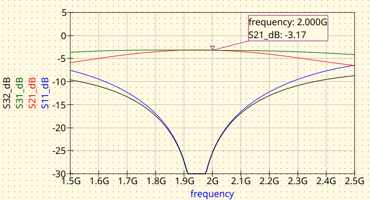
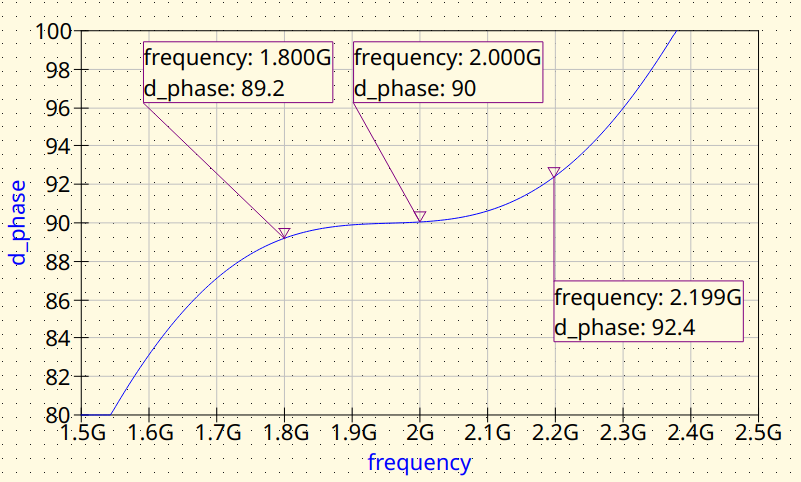
2.3 MS: Fine Tuning
The loading of the junctions need to be corrected to have the Branch-Line coupler working at 2000 MHz. The circuit variables are tuned for this.
Fined-tuned Branch-Line coupler (MS). Schematic
Fined-tuned Branch-Line coupler (MS). Magnitude response
Fined-tuned Branch-Line coupler (MS). Phase difference between outputs
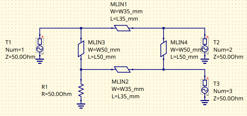
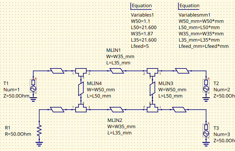
3. EM simulation
Once the microstrip model is good enough, then it’s convenient to validate it with an EM tool. EMerge software is particularly well suited for this. The reader is encourage to install EMerge from GitHub and give it a try.
The model definition is as follows:
And this is the Python script for running the simulation:
import matplotlib
matplotlib.use('WebAgg')
import matplotlib.pyplot as plt
import subprocess # Used to run the post-processing script
import emerge as em
import numpy as np
import time
from datetime import datetime

# ---------------------------------------------------------------------------
# PROJECT NAME
# ---------------------------------------------------------------------------
project_name = "Branch-Line Coupler 2000 MHz"


# ---------------------------------------------------------------------------
# Unit definitions
# ---------------------------------------------------------------------------
mm  = 1e-3         # m
mil = 0.0254 * mm  # meter per mil
MHz = 1e6          # Hz

# ---------------------------------------------------------------------------
# Substrate / material
# ---------------------------------------------------------------------------
er  = 3.55         # RO4003C relative permittivity
th  = 0.508        # [mm] (20 mil) Substrate thickness
tand = 0.0029      # Substrate tand

# ---------------------------------------------------------------------------
# Center frequency
# ---------------------------------------------------------------------------
f0_MHz = 2000;
f0 = f0_MHz*MHz    # centre frequency (Hz)

# ---------------------------------------------------------------------------
# Branch-line circuit model parameters
# ---------------------------------------------------------------------------
W50  = 1.1         # [mm] Trace width for 50-Ohm arms
W35  = 1.87        # [mm] Trace width for 35-Ohm arms

L35  = 22          # [mm] Quarter-wave length, 35-Ohm shunt arms
L50  = 22          # [mm] Quarter-wave length, 75-Ohm series arms

L_feed = 5         # [mm] Feed-line length

# ---------------------------------------------------------------------------
# Simulation setup
# ---------------------------------------------------------------------------
model = em.Simulation(project_name)
model.check_version("2.3.0")

# ---------------------------------------------------------------------------
# Frequency sweep
# ---------------------------------------------------------------------------
f_start = 100*MHz
f_stop = 3000*MHz
n_points = 40

# ---------------------------------------------------------------------------
# Material and PCB layouter
# ---------------------------------------------------------------------------
mat = em.Material(er=er, tand=tand, color="#488343", opacity=0.4)
pcb = em.geo.PCBNew(th, unit=mm, material=mat)

# ---------------------------------------------------------------------------
# Layout
# ---------------------------------------------------------------------------
pcb_margin = 25 # Space at both sides of the copper traces

# Port 1
x_P1 = 0
y_P1 = pcb_margin+W50/2

# Input feed line
pcb.new(x_P1, y_P1, W50, (-1, 0)).straight(L_feed)['p1']  # P1: input

# Input feedline tee
pcb.new(x_P1, y_P1, W50, (1, 0)).straight(W50)

# Input-side 35 Ohm line
pcb.new(x_P1+W50, y_P1, W35, (1, 0)).straight(L35)

# In-phase output tee
pcb.new(x_P1+W50+L35, y_P1, W50, (1, 0)).straight(W50)

# In-phase output port position
x_P2 = x_P1+W50+L35+W50
y_P2 = y_P1

# In-phase output feed line
pcb.new(x_P2, y_P2, W50,  (1, 0)).straight(L_feed)['p2']   # P2: in-phase output


# Isolated port
x_P3 = 0
y_P3 = pcb_margin+W50+L50+W50/2

# Isolated port feed line
pcb.new(x_P3, y_P3, W50, (-1, 0)).straight(L_feed)['p3']  # P3: Isolated port

# Isolated port tee
pcb.new(x_P3, y_P3, W50, (1, 0)).straight(W50)

# Isolated port-side 35 Ohm line
pcb.new(x_P3+W50, y_P3, W35, (1, 0)).straight(L35)

# Quadrature-output-side tee
pcb.new(x_P3+W50+L35, y_P3, W50, (1, 0)).straight(W50)

# Quadrature-output-side feed line
pcb.new(x_P3+W50+L35+W50, y_P3, W50, (1, 0)).straight(L_feed)

# Quadrature output port position
x_P4 = x_P3+W50+L35+W50
y_P4 = y_P3

pcb.new(x_P4, y_P4, W50, (1, 0)).straight(L_feed)['p4']   # P4: quadrature output

# Input-side 50 Ohm line joining the 35 Ohm branchline_post
pcb.new(x_P1+W50/2, y_P1+W50/2, W50, (0,1)).straight(L50)

# Output-side 50 Ohm line joining the 35 Ohm branchline_post
pcb.new(x_P2-W50/2, y_P2+W50/2, W50, (0,1)).straight(L50)


coupler = pcb.compile_paths(merge=True)

# ---------------------------------------------------------------------------
# Bounding box, dielectric and air
# ---------------------------------------------------------------------------
pcb.determine_bounds(topmargin=pcb_margin, bottommargin=pcb_margin)
diel = pcb.generate_pcb()
air  = pcb.generate_air(4 * th)

# ---------------------------------------------------------------------------
# Modal ports
# ---------------------------------------------------------------------------
p1 = pcb.modal_port(pcb['p1'], width_multiplier=5, height=4 * th)
p2 = pcb.modal_port(pcb['p2'], width_multiplier=5, height=4 * th)
p3 = pcb.modal_port(pcb['p3'], width_multiplier=5, height=4 * th)
p4 = pcb.modal_port(pcb['p4'], width_multiplier=5, height=4 * th)

# ---------------------------------------------------------------------------
# Solver settings
# ---------------------------------------------------------------------------
model.mw.set_resolution(0.2)
model.mw.set_frequency_range(f_start, f_stop, n_points)

# ---------------------------------------------------------------------------
# Assemble geometry
# ---------------------------------------------------------------------------
model.commit_geometry()

# ---------------------------------------------------------------------------
# Mesh refinement
# ---------------------------------------------------------------------------
model.mesher.set_boundary_size(coupler, 0.5 * mm, growth_rate=10)
model.mesher.set_face_size(p1, 0.5 * mm)
model.mesher.set_face_size(p2, 0.5 * mm)
model.mesher.set_face_size(p3, 0.5 * mm)
model.mesher.set_face_size(p4, 0.5 * mm)

# ---------------------------------------------------------------------------
# Mesh generation and visualisation
# ---------------------------------------------------------------------------
model.generate_mesh()
#model.view(plot_mesh=True)
model.view(plot_mesh=False)
# ---------------------------------------------------------------------------
# Boundary conditions
# ---------------------------------------------------------------------------
port1 = model.mw.bc.ModalPort(p1, 1, modetype='TEM')
port2 = model.mw.bc.ModalPort(p2, 2, modetype='TEM')
port3 = model.mw.bc.ModalPort(p3, 3, modetype='TEM')
port4 = model.mw.bc.ModalPort(p4, 4, modetype='TEM')

# ---------------------------------------------------------------------------
# Run solver
# ---------------------------------------------------------------------------
start_time = time.time()
data = model.mw.run_sweep(parallel=True, n_workers=8, frequency_groups=8)
run_time = (time.time() - start_time) / 60
print(f"Simulation completed in {run_time:.2f} minutes")

# ---------------------------------------------------------------------------
# Extract S-parameters (raw solver points)
# ---------------------------------------------------------------------------
grid = data.scalar.grid
f    = grid.freq

S11 = grid.S(1, 1)
S21 = grid.S(2, 1)
S31 = grid.S(3, 1)
S41 = grid.S(4, 1)
S42 = grid.S(4, 2)

# ---------------------------------------------------------------------------
# Vector fitting — supersampled plot
# ---------------------------------------------------------------------------
n_supersamples = 2001
f_fit   = np.linspace(f_start, f_stop, n_supersamples)
f_MHz = f_fit / 1e6    #  Scale for displaying the graphs
S11_fit = grid.model_S(1, 1, f_fit)
S21_fit = grid.model_S(2, 1, f_fit)
S31_fit = grid.model_S(3, 1, f_fit)
S41_fit = grid.model_S(4, 1, f_fit)
S42_fit = grid.model_S(4, 2, f_fit)

phase_S21   = np.angle(S21_fit, deg=True) # in-phase output
phase_S41   = np.angle(S41_fit, deg=True) # quadrature output
phase_diff  = phase_S21 - phase_S41

# ---------------------------------------------------------------------------
# 3-D field visualisation at f0
# ---------------------------------------------------------------------------
field = data.field.find(freq=f0)

model.display.add_object(diel)
model.display.add_object(coupler)
model.display.add_portmode(port1, k0=field.k0)
model.display.add_portmode(port2, k0=field.k0)
model.display.add_portmode(port3, k0=field.k0)
model.display.add_portmode(port4, k0=field.k0)
model.display.add_field(
    field.cutplane(0.5 * mm, z=-0.5 * th * mil).scalar('Ez', 'real'),
    symmetrize=True,
)
model.display.show()

# ---------------------------------------------------------------------------
# Export Touchstone
# ---------------------------------------------------------------------------
comments = [
    f"--- {project_name} ---",
    "Substrate: RO4003C",
    f"h = {th} mm",
    f"W50 = {W50} mm, W35 = {W35} mm",
    f"L35 = {L35} mm, L50 = {L50} mm",
    f"L_feed = {L_feed} mm",
    f"Run time = {run_time:.2f} min",
]

timestamp = datetime.now().strftime("%Y-%m-%d_%H-%M-%S")
grid.export_touchstone(project_name + "_EMerge_" + timestamp, custom_comments=comments)

# Save raw arrays for post-processing
np.savez(
    project_name + "_data.npz",
    f=f_fit, S11=S11_fit, S21=S21_fit, S31=S31_fit, S41=S41_fit, S42=S42_fit,
    phase_diff=phase_diff,
)


subprocess.run(["python", "branchline_post.py"], check=True)
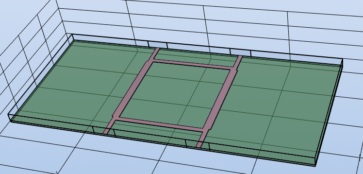
EMerge 3D model view
EMerge FEM simulation. Phase difference between outputs
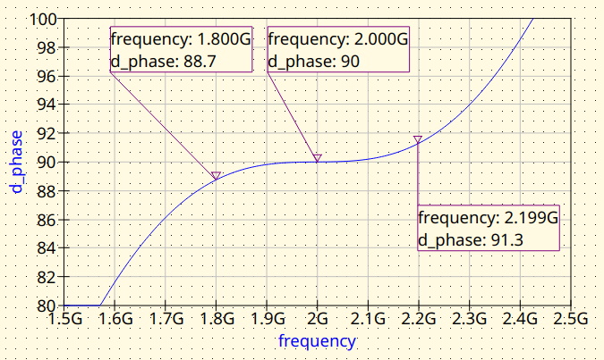
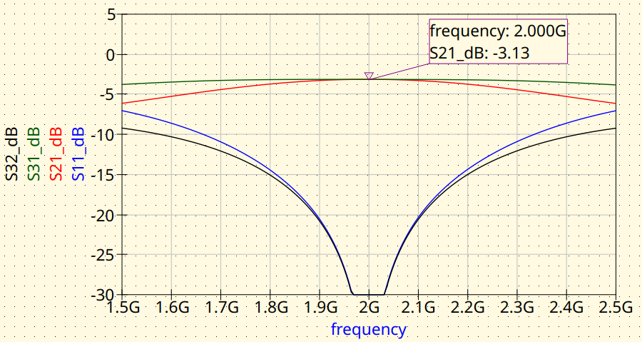
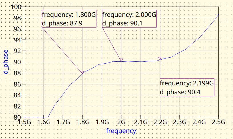
3.1 Use design variables from 2.2
First, the system is modelled using the design variables obtained from step 2.2 as the input
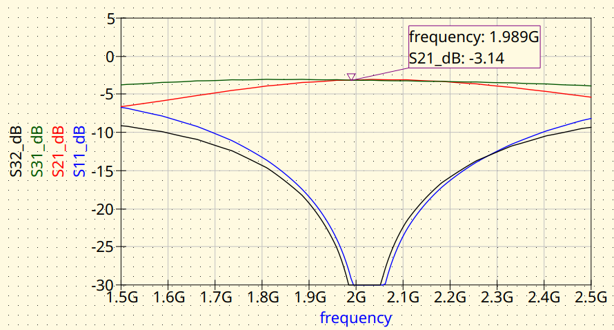
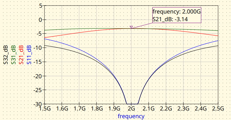
EMerge FEM simulation. Magnitude response.
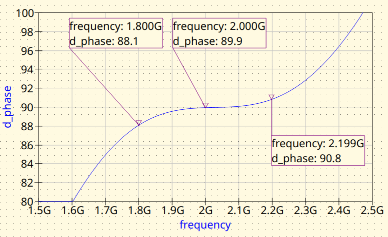
EMerge FEM simulation. Phase difference between outputs
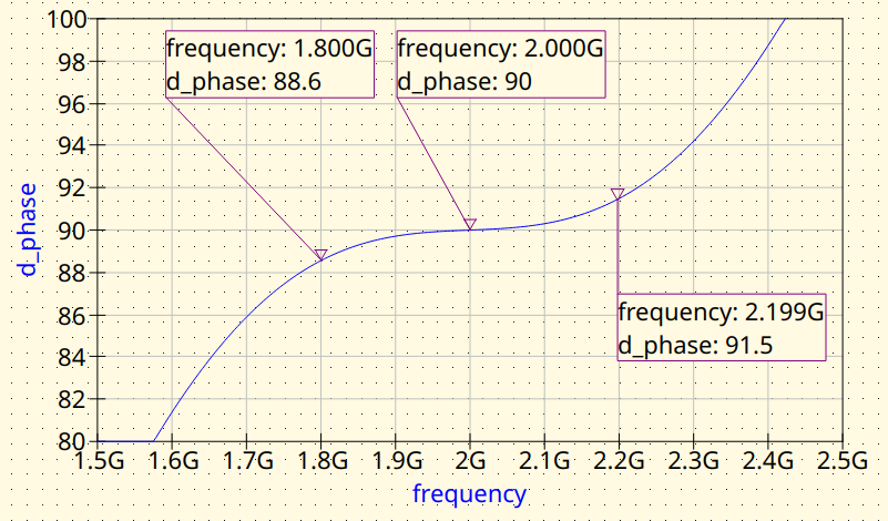
3.2 Fine-tuning
The reader may notice that the center frequency of the Branch-Line coupler is shifted towards high frequencies, so some retuning is needed.
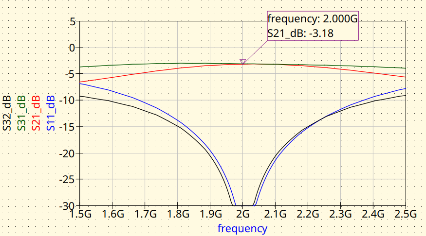
EMerge FEM simulation. Magnitude response.
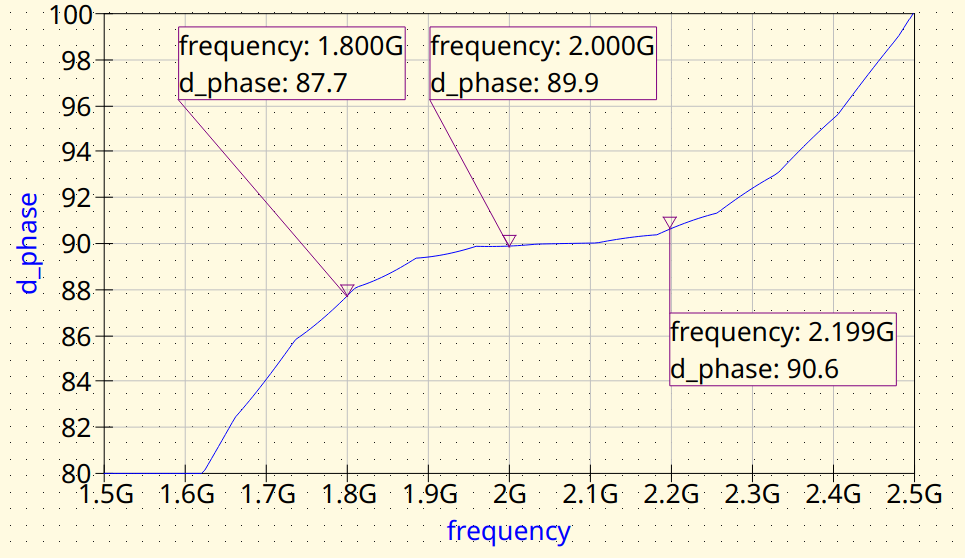
EMerge FEM simulation. Phase difference between outputs
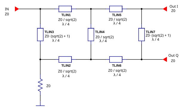
Double-Box Branch-Line Coupler
Let’s take a look at the double-box coupler. The design process is the same as shown before, so let’s skip that and jump into the results.
The script I’ve used is this:
import matplotlib
matplotlib.use('WebAgg')
import matplotlib.pyplot as plt
import subprocess  # Used to run the post-processing script
import emerge as em
import numpy as np
import time
from datetime import datetime

# ---------------------------------------------------------------------------
# PROJECT NAME
# ---------------------------------------------------------------------------
project_name = "Double-Box Branch-Line Coupler 2000 MHz"

# ---------------------------------------------------------------------------
# Unit definitions
# ---------------------------------------------------------------------------
mm  = 1e-3         # m
mil = 0.0254 * mm  # meter per mil
MHz = 1e6          # Hz

# ---------------------------------------------------------------------------
# Substrate / material
# ---------------------------------------------------------------------------
er   = 3.55   # RO4003C relative permittivity
th   = 0.508  # [mm] (20 mil) Substrate thickness
tand = 0.0029 # Substrate loss tangent

# ---------------------------------------------------------------------------
# Center frequency
# ---------------------------------------------------------------------------
f0_MHz = 2000
f0 = f0_MHz * MHz  # centre frequency (Hz)

# ---------------------------------------------------------------------------
# Branch-line circuit model parameters
#
# A double-box coupler is formed by cascading two single-box
# branch-line couplers:
#
#  P1 [50 Ω] ───── 35 Ω ────────── 35 Ω ─────── P2 [50 Ω]
#              |            |             |
#             121 Ω        35Ω           121 Ω
#              |            |             |
#  P3 [50 Ω] ───── 35 Ω ────────── 35 Ω ─────── P4 [50 Ω]
#
# ---------------------------------------------------------------------------
W50      = 1.1   # [mm] Trace width for 50 Ω feed lines
W35      = 1.9  # [mm] Trace width for 35 Ω series arms
W121     = 0.1 # [mm] Trace width for 121 Ω series arm


Lx  = 22.2     # [mm] Quarter-wave length. x-axis arms
Ly  = 22.2     # [mm] Quarter-wave length. y-axis arms

L_feed = 5   # [mm] Feed-line length

# ---------------------------------------------------------------------------
# Simulation setup
# ---------------------------------------------------------------------------
model = em.Simulation(project_name)
model.check_version("2.3.0")

# ---------------------------------------------------------------------------
# Frequency sweep
# ---------------------------------------------------------------------------
f_start  = 10  * MHz
f_stop   = 4000 * MHz
n_points = 40

# ---------------------------------------------------------------------------
# Material and PCB layouter
# ---------------------------------------------------------------------------
mat = em.Material(er=er, tand=tand, color="#488343", opacity=0.4)
pcb = em.geo.PCBNew(th, unit=mm, material=mat)

# ---------------------------------------------------------------------------
# Layout
#
# Coordinate conventions (same as single-box script):
#   x  →  horizontal (port-to-port direction along the top/bottom rails)
#   y  ↑  vertical   (between top and bottom rails)
#
# ---------------------------------------------------------------------------
pcb_margin = 25  # [mm] Board margin on all sides

# Port 1
x_P1 = 0
y_P1 = pcb_margin+W50/2

# ── TOP RAIL ─────────────────────────────────────────────────────────────
# P1 input feed line (exits left)
pcb.new(x_P1, y_P1, W50, (-1, 0)).straight(L_feed)['p1']

# Box1, first in-phase tee
pcb.new(x_P1, y_P1, W50, (1, 0)).straight(W121)

# Box-1 in-phase 35-Ω segment
pcb.new(x_P1 + W121, y_P1, W35, (1, 0)).straight(Lx)

# Tee between box 1 and box 2. In-phase branch
pcb.new(x_P1 + W121 + Lx, y_P1, W35, (1, 0)).straight(W35)

# Box-2 in-phase 35-Ω segment
pcb.new(x_P1 + W121 + Lx + W35, y_P1, W35, (1, 0)).straight(Lx)

# Tee between box 2 and in-phase output
pcb.new(x_P1 + W121 + Lx + W35 + Lx, y_P1, W50, (1, 0)).straight(W121)

# P2 feed line (in-phase output)
pcb.new(x_P1 + W121 + Lx + W35 + Lx + W121, y_P1, W50, (1, 0)).straight(L_feed)['p2']


# Port 3
x_P3 = 0
y_P3 = pcb_margin+W50+Ly+W50/2

# P3 input feed line (exits left)
pcb.new(x_P3, y_P3, W50, (-1, 0)).straight(L_feed)['p3']

# Box1, first quadrature-phase tee
pcb.new(x_P3, y_P3, W50, (1, 0)).straight(W121)

# Box-1 quadrature phase 35-Ω segment
pcb.new(x_P3 + W121, y_P3, W35, (1, 0)).straight(Lx)

# Tee between box 1 and box 2. quadrature phase branch
pcb.new(x_P3 + W121 + Lx, y_P3, W35, (1, 0)).straight(W35)

# Box-2 quadrature phase 35-Ω segment
pcb.new(x_P3 + W121 + Lx + W35, y_P3, W35, (1, 0)).straight(Lx)

# Tee between box 2 and quadrature output
pcb.new(x_P3 + W121 + Lx + W35 + Lx, y_P3, W50, (1, 0)).straight(W121)

# P4 feed line (quadrature output)
pcb.new(x_P3 + W121 + Lx + W35 + Lx + W121, y_P3, W50, (1, 0)).straight(L_feed)['p4']


# At this point we have two parallel lines between P1 and P2, and P3 and P4. We just need to add the 121 Ohm and 35 Ohm branches between the two compile_paths

pcb.new(x_P1+W121/2, y_P1+W50/2, W121, (0, 1)).straight(Ly)

pcb.new(x_P1 + W121 + Lx + W35/2, y_P1+W35/2, W35, (0, 1)).straight(Ly)


pcb.new(x_P1 + W121 + Lx + W35 + Lx + W121/2, y_P1+W50/2, W121, (0, 1)).straight(Ly)

coupler = pcb.compile_paths(merge=True)

# ---------------------------------------------------------------------------
# Bounding box, dielectric and air
# ---------------------------------------------------------------------------
pcb.determine_bounds(topmargin=pcb_margin, bottommargin=pcb_margin)
diel = pcb.generate_pcb()
air  = pcb.generate_air(4 * th)

# ---------------------------------------------------------------------------
# Modal ports
# ---------------------------------------------------------------------------
p1 = pcb.modal_port(pcb['p1'], width_multiplier=5, height=4 * th)
p2 = pcb.modal_port(pcb['p2'], width_multiplier=5, height=4 * th)
p3 = pcb.modal_port(pcb['p3'], width_multiplier=5, height=4 * th)
p4 = pcb.modal_port(pcb['p4'], width_multiplier=5, height=4 * th)

# ---------------------------------------------------------------------------
# Solver settings
# ---------------------------------------------------------------------------
model.mw.set_resolution(0.2)
model.mw.set_frequency_range(f_start, f_stop, n_points)

# ---------------------------------------------------------------------------
# Assemble geometry
# ---------------------------------------------------------------------------
model.commit_geometry()

# ---------------------------------------------------------------------------
# Mesh refinement
# ---------------------------------------------------------------------------
model.mesher.set_boundary_size(coupler, 0.5 * mm, growth_rate=10)
model.mesher.set_face_size(p1, 0.5 * mm)
model.mesher.set_face_size(p2, 0.5 * mm)
model.mesher.set_face_size(p3, 0.5 * mm)
model.mesher.set_face_size(p4, 0.5 * mm)

# ---------------------------------------------------------------------------
# Mesh generation and visualisation
# ---------------------------------------------------------------------------
model.generate_mesh()
model.view(plot_mesh=False)

# ---------------------------------------------------------------------------
# Boundary conditions
# ---------------------------------------------------------------------------
port1 = model.mw.bc.ModalPort(p1, 1, modetype='TEM')
port2 = model.mw.bc.ModalPort(p2, 2, modetype='TEM')
port3 = model.mw.bc.ModalPort(p3, 3, modetype='TEM')
port4 = model.mw.bc.ModalPort(p4, 4, modetype='TEM')

# ---------------------------------------------------------------------------
# Run solver
# ---------------------------------------------------------------------------
start_time = time.time()
data = model.mw.run_sweep(parallel=True, n_workers=8, frequency_groups=8)
run_time = (time.time() - start_time) / 60
print(f"Simulation completed in {run_time:.2f} minutes")

# ---------------------------------------------------------------------------
# Extract S-parameters (raw solver points)
# ---------------------------------------------------------------------------
grid = data.scalar.grid
f    = grid.freq

S11 = grid.S(1, 1)
S21 = grid.S(2, 1)
S31 = grid.S(3, 1)
S41 = grid.S(4, 1)
S42 = grid.S(4, 2)

# ---------------------------------------------------------------------------
# Vector fitting — supersampled plot
# ---------------------------------------------------------------------------
n_supersamples = 2001
f_fit  = np.linspace(f_start, f_stop, n_supersamples)
f_MHz  = f_fit / 1e6  # Scale for displaying the graphs

S11_fit = grid.model_S(1, 1, f_fit)
S21_fit = grid.model_S(2, 1, f_fit)
S31_fit = grid.model_S(3, 1, f_fit)
S41_fit = grid.model_S(4, 1, f_fit)
S42_fit = grid.model_S(4, 2, f_fit)

phase_S21  = np.angle(S21_fit, deg=True)  # in-phase output
phase_S41  = np.angle(S41_fit, deg=True)  # quadrature output
phase_diff = phase_S21 - phase_S41

# ---------------------------------------------------------------------------
# 3-D field visualisation at f0
# ---------------------------------------------------------------------------
field = data.field.find(freq=f0)

model.display.add_object(diel)
model.display.add_object(coupler)
model.display.add_portmode(port1, k0=field.k0)
model.display.add_portmode(port2, k0=field.k0)
model.display.add_portmode(port3, k0=field.k0)
model.display.add_portmode(port4, k0=field.k0)
model.display.add_field(
    field.cutplane(0.5 * mm, z=-0.5 * th * mil).scalar('Ez', 'real'),
    symmetrize=True,
)
model.display.show()

# ---------------------------------------------------------------------------
# Export Touchstone
# ---------------------------------------------------------------------------
comments = [
    f"--- {project_name} ---",
    "Substrate: RO4003C",
    f"h = {th} mm",
    f"W50 = {W50} mm, W35 = {W35} mm, W121 = {W121} mm",
    f"Lx = {Lx} mm, Ly = {Ly} mm",
    f"L_feed = {L_feed} mm",
    f"Run time = {run_time:.2f} min",
]

timestamp = datetime.now().strftime("%Y-%m-%d_%H-%M-%S")
grid.export_touchstone(project_name + "_EMerge_" + timestamp, custom_comments=comments)

# Save data for post-processing
np.savez(
    project_name + "_data.npz",
    # S-parameters
    f=f_fit, S11=S11_fit, S21=S21_fit, S31=S31_fit, S41=S41_fit, S42=S42_fit,
    phase_diff=phase_diff,
    # Substrate
    er=er, th=th, tand=tand,
    # Trace widths
    W50=W50, W35=W35, W121=W121,
    # Lengths
    Lx=Lx, Ly=Ly, L_feed=L_feed,
    # Frequency sweep
    f0_MHz=f0_MHz, f_start_MHz=f_start/MHz, f_stop_MHz=f_stop/MHz,
    # Run metadata
    run_time=run_time,
)

subprocess.run(["python", "postprocessing.py"], check=True)
Note that the magnitude response is much broader. The isolation is notably higher, and the phase difference between the outputs remains at 90° over a broader bandwidth. However, it exhibits slightly worse insertion loss on both outputs. This makes sense, given that we now have longer traces between the input and output.
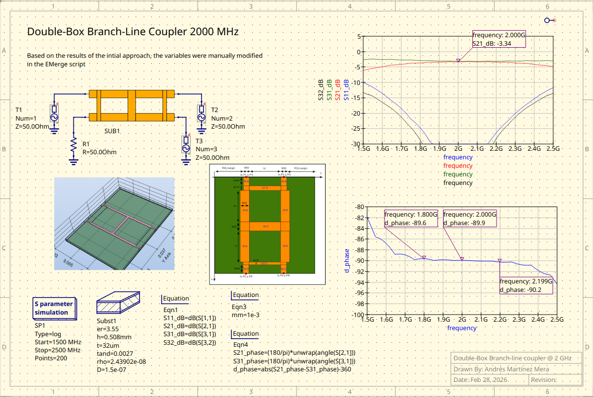
EMerge FEM simulation for the double-box design
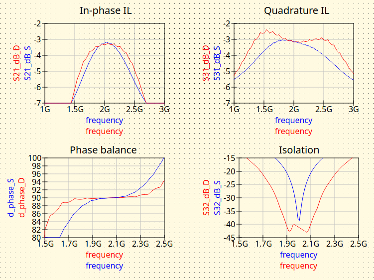
Comparison between single-box and double-box results